1.1.8.1.
Solution.
- 0.156
- 0.091
- 0.0007
- 1.356
=8+19 which gives 27=12*9 which gives 108=8^3 which gives 512=7.50/44.50 which gives approximately 0.1685, or approximately 16.85%=5780.23-5250 which gives $530.23=530.23/5250 which gives approximately 0.100996, or approximately 10.1%=5250*115.5% which gives exactly $6063.75=1000*103%*103% which gives $1060.90=1000*(103%)^2 gives the same result of $1060.90, because raising 103% to the second power means the same as multiplying 103% by itself two times.=1000*(103%)^15 which gives $1557.97 rounded to the nearest cent= B2*103% and the remaining cells are computed using the fill down feature.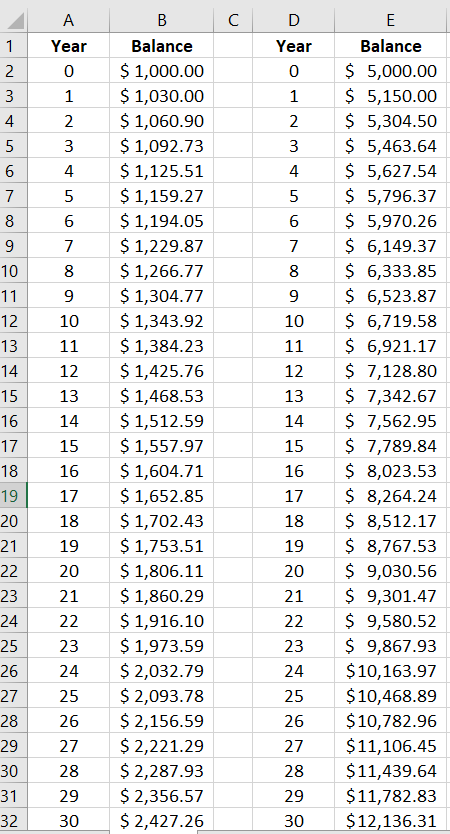
=FV(0.07/52,52*20,0,1000)
=FV(0.05/1,1*10,0,300)
=FV(0.04/52,52*25,0,10000)
=PV(0.05/4,4*4,0,20000)
=EFFECT(0.0375,12) \(=3.82\%\) and Ted =EFFECT(0.038,1) =3.8%. Bill has an effective rate of 3.82% and Ted has a rate of 3.8%.=FV(0.0375/12,5*12,0,6700)
=FV(0.038,5,0,6500)
2500*EXP(0.04*10)
=5000*EXP(0.045*5)
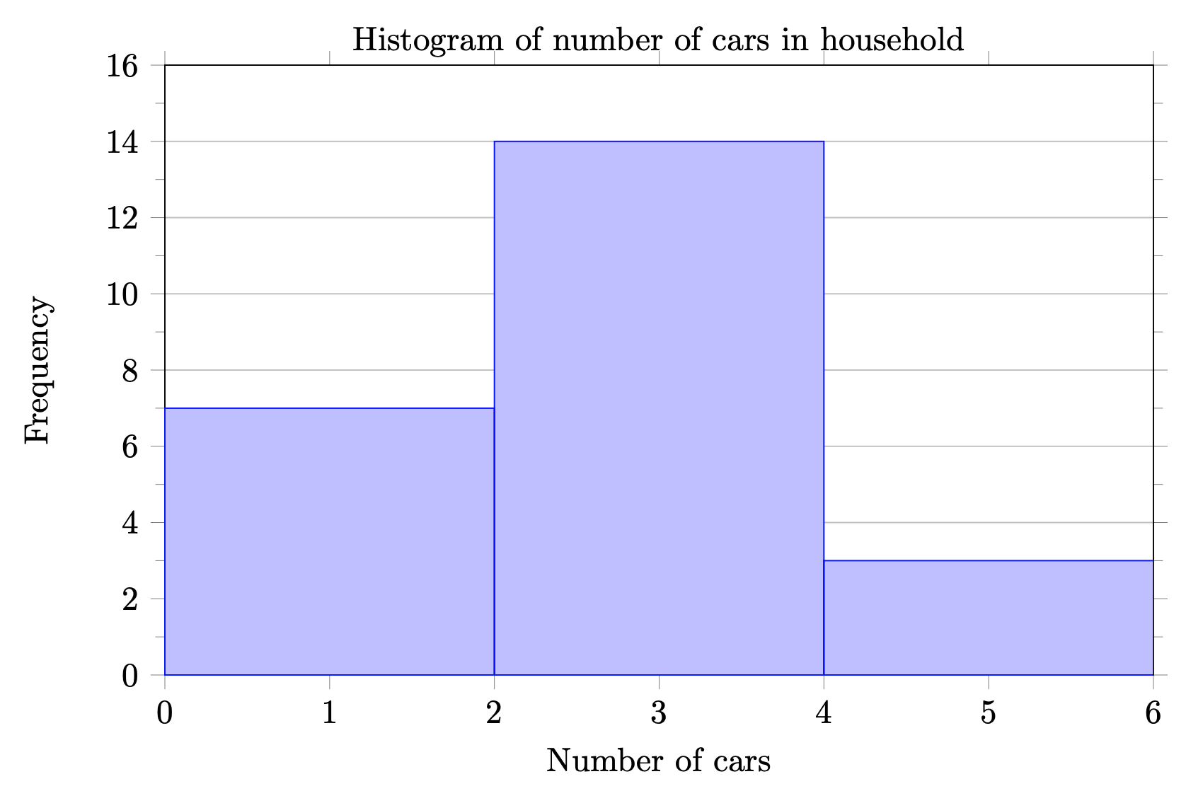
| Number of cars in household |
Frequency |
|---|---|
| 0-1 | 7 |
| 2-3 | 14 |
| 4-5 | 3 |
=average(7.50,25,10,10,7.50,8.25,9,5,15,8,7.25,7.50,8,7,12)=median(7.50,25,10,10,7.50,8.25,9,5,15,8,7.25,7.50,8,7,12)=average(15.2,18.8,19.3,19.7,20.2,21.8,22.1,29.4)=median(15.2,18.8,19.3,19.7,20.2,21.8,22.1,29.4)=average(A1:A40)=median(A1:A40)=average(A1:A40)=median(A1:A40)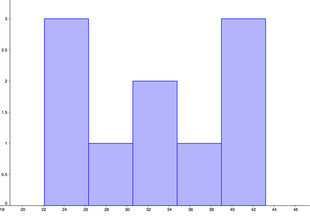
| 0, | 0, | 0, | 0, | 10 |
| 0, | 0, | 2, | 4, | 4 |
| 0, | 1, | 1, | 1, | 7 |
| 10, | 10, | 10, | 10, | 10 |
| 0, | 0, | 10, | 15, | 20 |
| 1, | 5, | 10, | 10, | 10 |
| Data Value | Deviation | Deviation Squared |
|---|---|---|
| \(7.5\) | \(7.5-9.8=-2.3\) | \((-2.3)^2=5.29\) |
| \(25\) | \(25-9.8=15.2\) | \((15.2)^2=231.04\) |
| \(10\) | \(10-9.8=0.2\) | \((0.2)^2=0.04\) |
| \(10\) | \(10-9.8=0.2\) | \((0.2)^2=0.04\) |
| \(7.5\) | \(7.5-9.8=-2.3\) | \((-2.3)^2=5.29\) |
| \(8.25\) | \(8.25-9.8=-1.55\) | \((-1.55)^2=2.4\) |
| \(9\) | \(9-9.8=-0.8\) | \((-0.8)^2=0.64\) |
| \(5\) | \(5-9.8=-4.8\) | \((-4.8)^2=23.04\) |
| \(15\) | \(15-9.8=5.2\) | \((5.2)^2=27.04\) |
| \(8\) | \(8-9.8=-1.8\) | \((-1.8)^2=3.24\) |
| \(7.25\) | \(7.25-9.8=-2.55\) | \((-2.55)^2=6.5\) |
| \(7.5\) | \(7.5-9.8=-2.3\) | \((-2.3)^2=5.29\) |
| \(8\) | \(8-9.8=-1.8\) | \((-1.8)^2=3.24\) |
| \(7\) | \(7-9.8=-2.8\) | \((-2.8)^2=7.84\) |
| \(12\) | \(12-9.8=2.2\) | \((2.2)^2=4.84\) |
| Min | Q1 | Median | Q3 | Max |
|---|---|---|---|---|
| $5 | $7.50 | $8 | $10 | $25 |
| Min | Q1 | Median | Q3 | Max |
|---|---|---|---|---|
| $5 | $7.50 | $8 | $10 | $25 |

| Min | Q1 | Median | Q3 | Max |
|---|---|---|---|---|
| 15.2 seconds | 19.05 seconds | 19.95 seconds | 21.95 seconds | 29.4 seconds |

| Min | Q1 | Median | Q3 | Max |
|---|---|---|---|---|
| 15 thousand dollars |
25 thousand dollars |
35 thousand dollars |
40 thousand dollars |
50 thousand dollars |

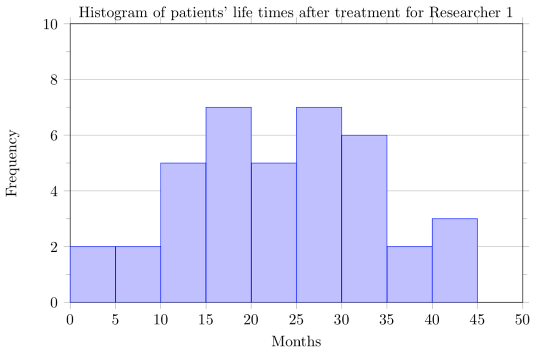
| Min | Q1 | Median | Q3 | Max |
|---|---|---|---|---|
| 3 months | 15 months | 24 months | 32.5 months | 47 months |
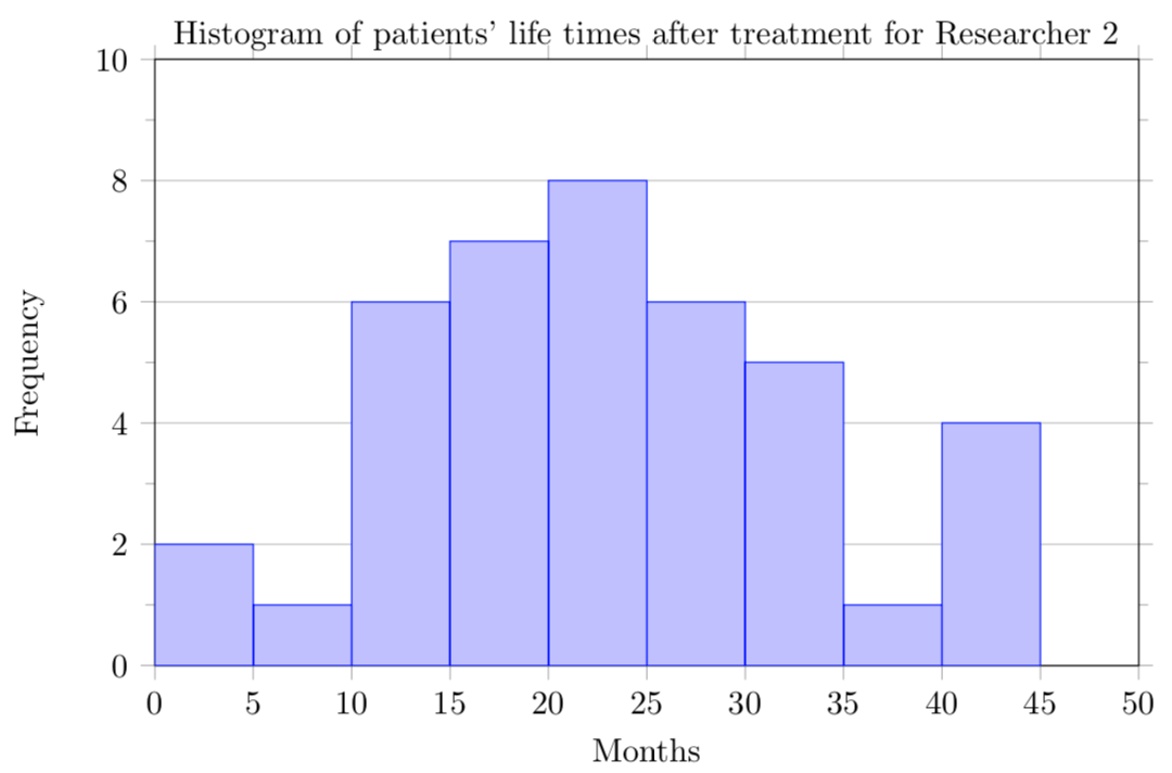
| Min | Q1 | Median | Q3 | Max |
|---|---|---|---|---|
| 2 months | 16 months | 22 months | 30 months | 44 months |

| Min | Q1 | Median | Q3 | Max |
|---|---|---|---|---|
| 22.1 chess pieces |
26.2 chess pieces |
32.6 chess pieces |
39.7 chess pieces |
43.2 chess pieces |
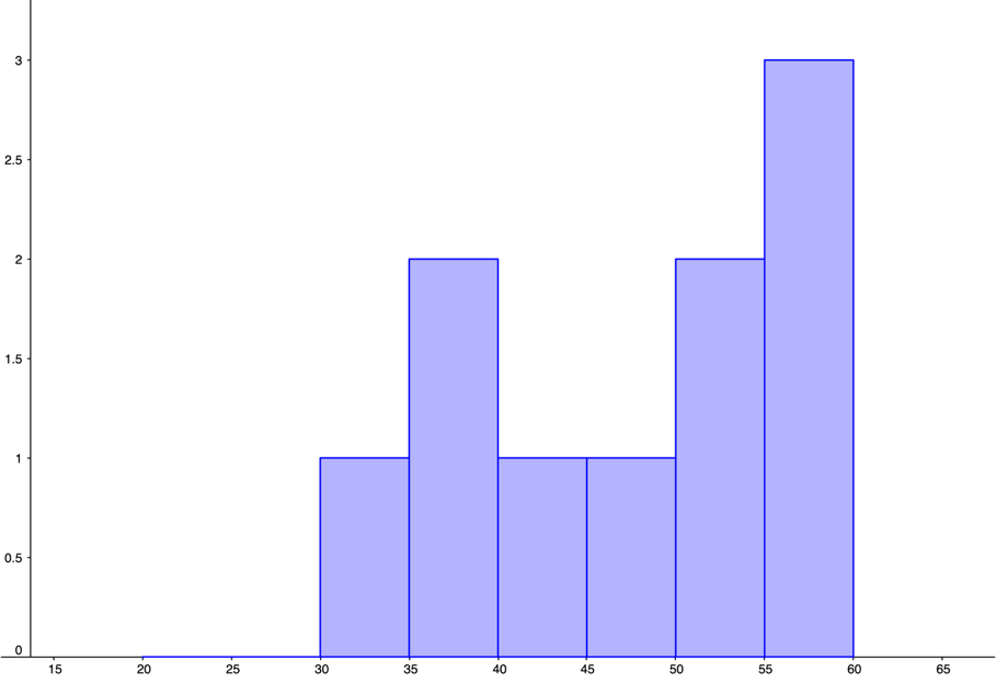
| Min | Q1 | Median | Q3 | Max |
|---|---|---|---|---|
| 32.5 chess pieces |
39.1 chess pieces |
48.4 chess pieces |
55.7 chess pieces |
57.7 chess pieces |
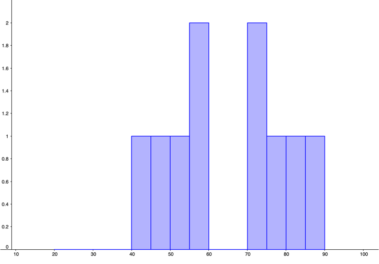
| Min | Q1 | Median | Q3 | Max |
|---|---|---|---|---|
| 40.1 chess pieces |
51.2 chess pieces |
64.6 chess pieces |
75.9 chess pieces |
85.3 chess pieces |


| Food Insecure | Not Food Insecure | Total | |
|---|---|---|---|
| Housing Insecure | 380 | 60 | 440 |
| Not Housing Insecure | 300 | 460 | 760 |
| Total | 680 | 520 | 1200 |
| Breakfast | No Breakfast | Total | |
|---|---|---|---|
| Floss | 12 | 49 | 61 |
| No Floss | 3 | 8 | 11 |
| Total | 15 | 57 | 72 |
| A | Not A | Total | |
|---|---|---|---|
| B | 10 | 20 | 30 |
| Not B | 20 | 25 | 45 |
| Total | 30 | 45 | 75 |
| Game/Software | No Game/Software | Total | |
|---|---|---|---|
| Computer | 10% | 5% | 15% |
| No Computer | 15% | 70% | 85% |
| Total | 25% | 75% | 100% |
| Hardcover | Paperback | Total | |
|---|---|---|---|
| Fiction | 13 | 59 | 72 |
| Nonfiction | 15 | 8 | 23 |
| Total | 28 | 67 | 95 |
| Die roll | Gold | Silver | Black |
|---|---|---|---|
| Outcome | $3 | $2 | -$1> |
| Probability | \(3/37\) | \(6/37\) | \(28/37\) |
| Die roll outcome | 1, 2, 3, or 4 | 5 | 6 |
|---|---|---|---|
| Outcome | $5 | $0 | -$2 |
| Probability | \(1/6\) | \(1/6\) | \(4/6\) |
| Number of voters | 3 | 3 | 1 | 3 | 2 |
|---|---|---|---|---|---|
| 1st choice | A | A | B | B | C |
| 2nd choice | B | C | A | C | A |
| 3rd choice | C | B | C | A | B |
| State | Population | Number of Representatives |
Number of Senators |
Number of Electors |
|---|---|---|---|---|
| Gandhi | 450,000 | 9 | 2 | 11 |
| Mandela | 150,000 | 3 | 2 | 5 |
| Gbowee | 600,000 | 12 | 2 | 14 |
| Total | 1,200,000 | 24 | 6 | 30 |
| State | Population | Number of Representatives |
Number of Senators |
Number of Electors |
|---|---|---|---|---|
| Tamez | 280,000 | 7 | 2 | 9 |
| Teters | 200,000 | 5 | 2 | 7 |
| Herrington | 400,000 | 10 | 2 | 12 |
| Osawa | 360,000 | 9 | 2 | 11 |
| Total | 1,240,000 | 31 | 8 | 39 |
| State | Votes for Candidate A |
Votes for Candidate B |
Number of Electoral Votes for A |
Number of Electoral Votes for B |
|---|---|---|---|---|
| Gandhi | 216,000 | 234,000 | 0 | 11 |
| Mandela | 37,500 | 112,500 | 0 | 5 |
| Gbowee | 489,450 | 110,550 | 14 | 0 |
| Total Votes | 742,950 | 457,050 | 14 | 16 |
| State | Votes for Candidate A |
Votes for Candidate B |
Number of Electoral Votes for A |
Number of Electoral Votes for B |
|---|---|---|---|---|
| Tamez | 95,480 | 184,250 | 0 | 9 |
| Teters | 104,200 | 95,800 | 7 | 0 |
| Herrington | 203,600 | 196,400 | 12 | 0 |
| Osawa | 46,080 | 313,920 | 0 | 11 |
| Total Votes | 449,360 | 790,640 | 19 | 20 |
| State | Population | Number of Representatives |
Number of Senators |
Number of Electors |
Electoral Votes per 50,000 people |
|---|---|---|---|---|---|
| Gandhi | 450,000 | 9 | 2 | 11 | 1.22 |
| Mandela | 150,000 | 3 | 2 | 5 | 1.67 |
| Gbowee | 600,000 | 12 | 2 | 14 | 1.17 |
| State | Population | Number of Representatives |
Number of Senators |
Number of Electors |
Electoral Votes per 50,000 people |
|---|---|---|---|---|---|
| Tamez | 280,000 | 7 | 2 | 9 | 1.29 |
| Teters | 200,000 | 5 | 2 | 7 | 1.40 |
| Herrington | 400,000 | 10 | 2 | 12 | 1.20 |
| Osawa | 360,000 | 9 | 2 | 11 | 1.22 |
