Distinguish between exponential and linear growth.
Develop exponential functions to model growth and decay in context.
Interpret exponential models and their outputs in context.
Subsection2.3.1Exponential Growth and Decay Models
The next growth model we will examine is exponential growth. Linear growth occurs when a population increases by the same amount in each unit of time. Exponential growth happens when an initial population increases by the same percentage or factor in each unit of time.
For example, consider a town of 1,000 people that is experiencing a population boom due to an abundance of jobs and affordable housing. The population grows exponentially by 20% per year. After one year, there will be \(1000+0.20\cdot 1000=1200\) people. The next year, the population will grow by 20% of 1,200 people, so there will be \(1200+0.20\cdot 1200=1440\) people. The year after that, there will be \(1440+0.20 \cdot 1440=1728\) people.
Let’s compare this population that start with 1,000 people and grows by 20% per year, which is exponential growth, with a population that starts with 1,000 people and grows by 200 people per year, which is linear growth.
Table2.3.1.Linear and Exponential Growth
Year
Population Subject to Linear Growth
Population Subject to Exponential Growth
0
1000
1000
1
1200
1200
2
1400
1440
3
1600
1728
4
1800
2074
5
2000
1488
10
3000
6192
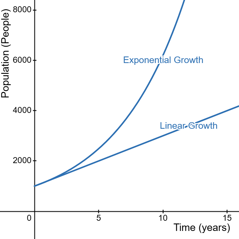
Please notice that at first, the populations according the the two models are very close, but as time goes on, the exponential model becomes increasingly larger than the linear model. This is because the linear model grows by the same amount in each unit of time while the exponential model grows by an increasing amount in each unit of time. We can use a graph to help visualize the difference between linear and exponential growth.
Figure2.3.2.Linear and Exponential Growth
Example2.3.3.Duck Population.
A population of ducks in a park grows exponentially. Initially, there were 200 ducks, and the population grows by 10% per month.
Find the population after one month.
Find the population after two months.
Find the population after ten months.
Develop a formula for the duck population after \(t\) months.
Solution.
After one month, the population will have increased by \(0.10\cdot200=20\text{.}\) The new population is 220 ducks.
Important Observation: We just calculated \(200+0.10\cdot200\text{.}\) Factoring out the 200, this is the same as \(200(1+0.10)\) which can be simplified to \(200(1.1)\)
In the second month, the population begins at 220 ducks and increases by \(0.10*220=22\text{.}\) The new population is 242 ducks.
Important Observation: Using the same logic above, we could have calculated this as \(220(1.1)\text{.}\) Recall that we found 220 by multiplying \(200(1.1)\text{,}\) so the population after 2 months will be \(200(1.1)(1.1)=242\text{.}\)
Consider the "important observations" in the first parts of this example. To find the population after ten months, we can start with the initial population of 200 ducks and multiply by a factor of 1.1 for each month. Using exponential form, that is, \(200(1.1)^{10}\approx 519\) ducks.
Generalizing the answer to the previous part of this exercise, we obtain \(P(t)=200(1.1)^{t}\text{.}\)
We can generalize the solution to the above example to develop a formula for exponential growth. In the function \(P(t)=200(1.1)^{t}\text{,}\) what do the 200, the 1.1, and the \(t\) represent in context?
200 is the initial or starting duck population. Recall from Section 2.1 that we use \(P_0\) to represent the initial value.
We found the value 1.1 by adding 1 and 0.10, which represents the 10% exponential growth rate. We can also think of 1.1=1.10 as meaning that after each month there are 110% as many ducks as there were in the previous month. We will use the variable \(r\) to represent the exponential growth rate. So we have \(1.1=1+0.10=1+r\text{.}\)
We will continue to use the variable \(t\) to represent time using units that are appropriate to the situation, such as years, months, days, etc.
Putting this information together, we can build the exponential growth model \(P(t)=P_0(1+r)^{t}\text{.}\)
Develop an exponential model for the population of a city with an initial population of 2,000,000 people and is losing 4% of its population each year.
Solution.
For simplicity, we can choose to measure the population in millions, so \(P_0=2\text{.}\)
We will measure time in years since we are given an annual rate. Because the town is losing population, the growth rate is negative. Thus, \(r=-0.04\text{.}\)
The resulting equation of the form \(P(t)=P_0(1+r)^{t}\) is
The average inflation rate in October, 2024, was 2.6% per year. If a new car cost $35,000 in October, 2024, how much would it cost to buy the same kind of car new in October, 2030? You may assume that the price of new cars will increase with inflation.
Solution.
Let’s use \(t=0\) to denote October, 2024, and count time in years. The initial value is \(P_0=35000\) and the growth rate is \(r=2.6\%=0.026\text{.}\)
The value of the car after \(t\) years can be found using the formula \(P(t)=35000(1+0.026)^{t}
\text{.}\) We can simplify this expression to \(P(t)=35000(1.026)^{t}\text{.}\)
We are looking for the population in the year 2030, which is \(t=2030-2024=6\text{.}\) Therefore, in 2030 a new car would cost
In the early days of an epidemic or pandemic, disease spreads according to an exponential model. On March 13, 2020, Kitsap County, Washington, had a total of seven confirmed positive COVID-19 cases. By March 22 of that year, there were 31. If the disease continued to spread at the same exponential rate, how many cases would have accumulated by March 27? How many by April 27? (Round the growth rate to four decimal places.)
Solution.
Let’s start by writing down what we know and what we need to find:
We are told that this is exponential growth, so we will use the formula \(P(t)=P_0(1+r)^{t}\) where \(P(t)\) is the total of accumulated positive cases at time \(t\text{.}\)
The initial value is \(P_0=7\) where \(t=0\) corresponds to March 13, 2020.
On March 22, there were 31 total cases. Measuring time in days, March 22 is day \(t=22-13=9\text{.}\) Then we can translate the number of cases on March 22 into mathematical notation as \(P(9)=31\text{.}\)
We do not know the growth rate \(r\text{,}\) but we can set up an equation using the above information to find it.
Once we finish building our function, we can use the function to find the predicted total number of positive COVID tests on March 27 and April 13 of 2020.
To find the value of the growth rate, \(r\text{,}\) we will plug in the values of \(P_0\) and \(P(9)\) and solve the resulting equation as follows:
To calculate the ninth root on a calculator, you can use the nth root button which is likely to look like \(\sqrt[n]{}\text{.}\) The keyboard shortcut in the DESMOS calculator is nthroot.
We can simplify to \(P(t)=7\left(1.1798\right)^{t}\text{.}\)
Finally, we can use this function to answer the questions.
March 27 is day \(t=27-13=14\text{.}\) TO find the number of cases on day 14, we evaluate \(P(14)=7(1.1798)^{14}\approx71\) cases. (In reality, there were 70 cases on this date, so the prediction is very close!)
April 13 is exactly one month after March 13. Since there are 31 days in march, this is day \(t=31\text{.}\) To find the number of cases accumulated on this day, we evaluate \(P(31)=7(1.1798)^{31}\approx1178\) cases.(In reality, there were only 135 cases on this date. We may infer that the infection had already stopped spreading at an exponential rate.)
$0
Example2.3.8.Exponential Decay.
Hydrogen-3, also known as tritium, is a radioactive isotope of hydrogen and a byproduct of nuclear energy production. It decays exponentially with a half-life of 12 years, meaning that after 12 years, the amount of tritium in a sample is reduced by half. (The decayed tritium doesn’t just disappear; it is converted to helium, releasing an electron and a small amount of radiation in the process.) If there are 40 grams of tritium now, how much will be left in 6 years? Round the growth rate to six decimal places.
Solution.
First we will build a model of the form \(P(t)=P_0(1+r)^{t}\) where time is measured in years and the \(P\) is measured in grams. We are given that \(P_0=40\text{.}\)
Since the half-life of tritium is 12 years, we know that after 12 years, we will be left with half of our 40-gram starting amount.
Therefore, there are 28g of tritium remaining after 6 years.
Comment: It would be very tempting to observe that 6 years is half of a half-life. If 20 grams of tritium decay in 12 years, why don’t we lose 10 grams of tritium in 6 years, leaving 30 grams? This type of proportional reasoning only works with linear models where the value changes by the same amount in each unit of time. With exponential decay, the rate of change is a percentage of the amount of substance remaining at each point in time. So the rate of change is not constant.
Subsection2.3.2When Good Models Go Bad
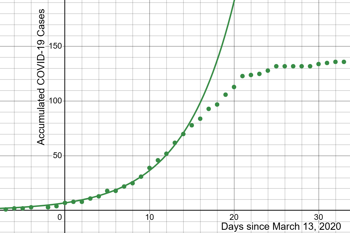
Recall that in Example 2.3.7, the exponential model worked well in predicting \(P(14)\text{,}\) the total confirmed positive cases by March 22, but the prediction for \(P(31)\text{,}\) the total confirmed positive cases by April 13 was not even close to the actual value. The graph below shows the number of accululated cases by day and the graph of the function we built to model the situation.
Figure2.3.9.Total accumulated covid cases in Kitsap County, WA, and exponential model \(P(t)=7(1.1798)^{t}\text{.}\) Data obtained from Kitsap Public Health Department.
The function \(P(t)=7(1.1798)^{t}\) closely models the number of cases very early in the pandemic, but the model appears to break down after about \(t=15\) which is March 25 when the number of cases appears to start leveling off. This could be related to the "Stay Home, Stay Healthy" executive order announced on March 23, 2020, which banned social gatherings and closed all but essential businesses to in-person work.
In practice, all exponential models break down eventually. It is not feasible for something to keep growing forever. Populations will run out of space or resources, and conditions will change.
Like linear models, exponential models are useful tools for short-term predictions but should be used with caution for long-term predictions.
Subsection2.3.3Special Cases
The general formula \(P(t)=P_0(1+r)^{t}\) can be applied broadly in exponential growth and decay applications. However, with a few minor adjustments, we can create special models to save time in some common situations.
In Example 2.3.8, we found that \(1+r=\sqrt[12]{\frac{1}{2}}\text{.}\) Using this exact value, we can write the function as
Recall the exponent rules that \(\sqrt[n]{x}=x^{\frac{1}{n}}\) and \((x^{m})^{n}=x^{m \cdot n}\text{.}\) Using these rules, we can simplify the function as follows:
The model \(P(t)=40\left(\frac{1}{2}\right)^{\frac{t}{12}}\) shows both the initial value and the half-life of 12 years in the function!
In general, we can model exponential decay with the formula \(P(t)=P_0 \left(\frac{1}{2}\right)^{\frac{t}{h}}\) where \(P_0\) is the initial amount and \(h\) is the half-life.
Example2.3.10.Use the Half-Life Model to Build a Function.
A sample of a radioactive substance with half-life 27 seconds has an initial amount of 12 kilograms. Write an exponential function to model the amount of the substance in kilograms remaining after \(t\) seconds.
Answer.
P(t)=12 \left( \frac{1}{2}right)^{\frac{t}{27}}
Example2.3.11.Half-Life Model Interpretation.
A sample of a radioactive substance decays according to the model \(P(t)=50\left(\frac{1}{2}\right)^{\frac{t}{4}}\text{,}\) where \(P\) is measured in grams and \(t\) is measured in hours. What is the inital amount of the substance, and what is the half-life?
Answer.
The initial amount is \(50\) grams, and the half-life is \(4\) hours.
In population studies, it is common to focus on the doubling time, or the amount of time it takes for a population to double in size. We can make a simple adjustment on the half-life model to develop a doubling-time model:
We can generalize the half-life and doubling-time models to apply to any multiplier. If a value is multiplied by \(M\) every \(T\) units of time, we can model the situation with an exponential function of the form \(P(t)=P_0 \left(M\right)^{\frac{t}{T}}\text{.}\)
Example2.3.13.Using a Multiplier.
A new house was sold for $400,000 in 2011. In 2021 the house was worth $600,000. If home values continue to grow exponentially at the same relative rate, what will the home’s value be in 2029? Round to the nearest dollar.
Solution.
For simplicty, we will measure the value in thousands of dollars and time in years since 2011. Thus, \(P_0=400\text{.}\)
The multiplier is \(M=\frac{600}{400}=1.5\text{,}\) and it took \(T=2021-2011=10\) years. We will use the model
To find the value of the house in the year 2029, which is time \(t=2029-2011=18\text{,}\) we evaluate \(P(18)=600\left(1.5\right)^{\frac{18}{10}}\approx1244.846\text{.}\)
Remembering that the value we found is in thousands of dollars, we conclude that the house will be worth about $1,244,846 in the year 2029.
Note that you could also have taken the approach of Example 2.3.7 and other examples in which we used a model of the form \(P(t)=P_0 (1+r)^{t}\text{,}\) which required several algebraic steps to first solve for the value of \(r\text{.}\) Both approaches will work equally well!