Linear growth occurs when quantities increase or decrease at a constant rate over time, which is common in real-life scenarios like budgeting, population changes, and transportation. Understanding linear growth helps us make predictions, solve problems, and analyze trends in fields like science, economics, and everyday decision-making.
Objectives
Students will be able to:
Identify linear growth in context.
Interpret linear growth models.
Use linear growth models to solve applied problems.
Subsection2.1.1Linear Growth Models
A linear growth model is an equation used to represent something that changes by the same amount in each unit of time. We use the term growth even in situations where a quantity is decreasing by the same amount in each unit of time. (It is growing by a negative amount.) Following are some examples of linear growth:
A tree is 4 feet tall when it is planted, and it grows 2 feet each year.
The value of a car is $38,000 when new, and the value decreases by $2,000 each year.
The total cost to repair a dishwasher is $100 plus $80 for each hour of labor.
The population of a small town is 4,070 people in the year 2025, and it is increasing by 5 people per year.
In each example, the value changes by the same amount in each unit of time: 2 feet each year, $2,000 each year, $80 each hour, and 5 people each year.
Consider the tree that starts out 4 feet tall and grows 2 feet each year. After 1 year, it will be 6 feet tall, after 2 years it will be 8 feet tall, after 3 years it will be 10 feet tall, and so on.
We can demonstrate the growth pattern with a table and a graph.
Table2.1.1.Tree growth over time
Time (yrs)
Height (ft)
0
4
1
6
2
8
3
10
4
12
5
14
6
16
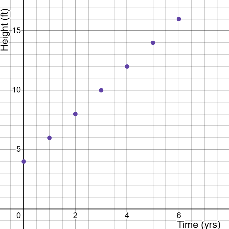
By convention, we put time on the horizontal axis when dealing with growth models. Plotting the points in the table above results in the following graph.
Figure2.1.2.Linear growth pattern
Note that if we connect the data points, the result would be a straight line, which is why we call this type of trend linear growth.
Imagine that we wanted to predict the height of the tree after 20 years. We would start with the initial height of 4 feet and add 2 feet 20 times. Mathematically, this is \(4+2(20)=84\text{.}\)
Generalizing, we can obtain a formula for the height of the tree after \(t\) years:
\begin{equation*}
H(t)=4+2t.
\end{equation*}
Recall from algebra classes that \(H(t)\) indicates function notation, not multiplication. We read it as "\(H\) of \(t\)".
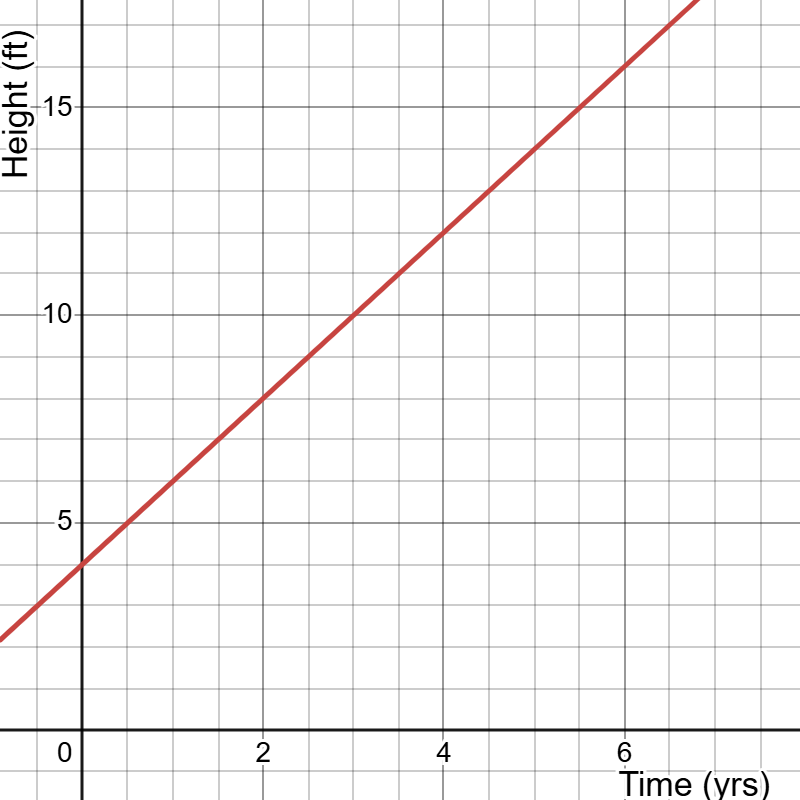
As expected, the graph of \(H(t)=4+2t\) is a straight line.
Figure2.1.3.Graph of \(H(t)=4+2t\text{.}\)
Using a similar approach we can write linear functions to model the remaining examples mentioned above:
The value of the car that starts out at $38,000 and loses $2,000 in value each year can be modeled with the function \(V(t)=38\,000-2\,000t
\text{.}\)
The $100 plus $80 per hour cost to repair the dishwasher can be modeled with the function \(C(t)=100+80t\) where \(t\) is measured in hours.
The population of the town that starts at 4,070 and grows by 5 people per year since the year 2025 can be modeled with the function \(P(t)=4\,070+5t\) where \(t\) is the number of years since 2025.
Linear Growth Model.
Linear growth can be modeled with functions of the form
\begin{equation*}
P(t)=P_0+Dt
\end{equation*}
where
\(P(t)\)
is the amount at time \(t\text{,}\)
\(P_0\)
is the initial amount,
\(D\)
is the common difference or growth rate, which is the amount of growth in each unit of time, and
t
is the amount of time.
Note that \(D\) can be negative.
Is the linear growth model equivalent to the slope-intercept form of a line \(y=mx+b\) from middle school and high school algebra classes? Yes, it is!
The general linear growth model equation above uses the letter \(P\) because population models are one of the more common applications.
The constant \(P_0\) can be read "P sub zero", "P zero", or "P naught", and it represents the population or value at time zero. When viewing the graph, the point where line intersects the vertical or y-axis is called the y-intercept. Its coordinates are \((0,P_0)\text{.}\)
Recall that linear growth occurs when a value changes by the same amount in each unit of time, and growth can be either positive or negative depending on whether the value is increasing or decreasing.
Example2.1.4.
Identify whether each scenario is an example of linear growth. If it is linear growth, find the initial value, the common difference or growth rate, and the equation.
A projectile starts at ground level. It reaches its maximum height of 40 feet after two seconds and lands after four seconds. Is the height of the projectile a linear function of time?
Solution.
The height increases and then decreases. Therefore, it does not have a constant rate of change, and it is not linear. (It is quadratic.)
The population of a small town is 1,042 people in the year 2015, and the population grows by 19 people per year. Is the population a linear function of time?
Solution.
The growth rate is a constant 19 people per year, so this is linear growth. If we let \(t=0\) be the year 2015, then the initial value is \(P_0=1\,042\) and the growth rate is 19 people per year.
The equation is \(P(t)=1042+19t\text{.}\)
The population of a small town is 1,042 people in the year 2015, and the population grows by 2.9% per year. Is the population a linear function of time?
Solution.
The first year, the population grows by 2.9% of 1042, which is about 30 people or a new population of 1072 people. The second year, the population grows by 2.9% of 1072, which is about 31 people. The amount of growth is not the same, so this is not linear growth. (It is exponential growth.)
For tax and planning purposes, a business estimates that a tractor purchased for $28,000 will be worth $0 after seven years of use. It depreciates by the same amount each year. Is the reported value of the tractor a linear function of time?
Solution.
This is linear because the value depreciates by the same amount each year. The initial value is \(V_0=28\,000\) dollars. The common difference \(D=-\frac{28\,000}{7}=-4\,000\) dollars each year. The resulting equation is
where \(V\) is the value in dollars after \(t\) years.
The population of Poulsbo, Washington, was about 9,300 people in 2010, about 12,000 people in 2020, and about 12,200 people in 2024. Is the population of Poulsbo a linear function of time?
Solution.
To determine if this is linear growth, we will determine the growth rates from 2010 to 2020 and from 2020 to 2024 to see if they are the same.
From 2010 to 2020, the population grew by \(12\,000-9\,300=2700\) people in 10 years, which is a growth rate of \(2700/10=270\) people per year.
From 2020 to 2024, the population grew by 200 people in four years, which is a growth rate of \(200/4=50\) people per year. Since the growth rates are not approximately equal, the population of Poulsbo is not growing linearly.
Example2.1.5.
Kobi drives an average of 1,050 miles each month. They just purchased a used car with 43,000 miles on the odometer.
Develop a linear model to represent the number of miles on the odometer after \(t\) months.
Solution.
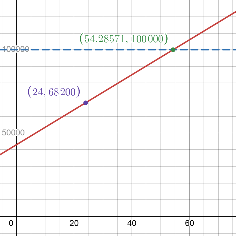
Measuring time in months since Kobi purchased the car, the initial value is \(P_0=43000\text{.}\) The common difference is \(d=1050\) miles per month. Therefore, we can build the model
to solve the problem. Using the method demonstrated in Appendix D, we obtain the following graph.
The mileage reaches 100,000 miles at \(t=54.28571\text{,}\) which is about 54 months.
Subsection2.1.2When Good Models Go Bad
When using any mathematical model, it is important to consider how long the model will be valid. At the beginning of this section, we discussed the example of a tree that grows two feet per year from an initial height of four feet. Is it reasonable to think that the tree will grow about two feet each year forever? Is it reasonable to think that it was growing by two feet per year before it was planted at time \(t=0\text{?}\) Probably not. It is likely that the tree will grow by two feet per year for several years, perhaps five to ten or even twenty years, before the rate of growth slows down. If the tree is left to live a natural lifesapn, eventually it will stop growing, die, and decompose. The model \(H(t)=4+2t\) may be useful for a limited interval of time, such as five to ten years before its validity breaks down.
How far into the future will a linear model serve as a valid predictor? Engineers and statisticians use error analysis methods involving calculus to find approximate answers to this question. In this book, we will use knowledge of the examples at hand to estimate realistic bounds.
Example2.1.6.
An espresso machine for a coffee stand is purchased for $15,000. For tax and planning purposes, the owner reports that the machine will depreciate linearly over ten years. Find a model to represent the reported value after \(t\) years and estimate the interval over which the model will be valid.
Solution.
The starting value of the machine is \(V_0=15000\text{.}\) The rate of change is
Therefore, we can use the model \(V(t)=15000-1500t\) where \(t\) is the number of years since the espresso machine was purchased and \(V\) is the reported value in dollars.
It does not make sense to consider the value of the machine before it was purchased or after its value has dropped to $0. Therefore, this model should be valid for values of \(t\) between \(t=0\) and \(t=10\text{.}\) This is only an estimate because the machine could break earlier or changing economic conditions could raise or lower the reported value.
Example2.1.7.
The price of a one-term subscription to an online mathematics homework system was $100 in 2019. The price has been increasing linearly, and the same subscription cost $142 in 2025.
Find a model to represent the price \(P\) of the subscription \(t\) years after the year 2019.
Based on the situation, over which of following intervals for \(t\) would you anticipate that this model will be valid?
\(t=0\) to \(t=1\)
\(t=-5\) to \(t=15\)
\(t=-100\) to \(t=100\)
\(\displaystyle t\gt0\)
Solution.
The starting value is given to be $100.
Before finding the rate of change, we note that the year 2025 is \(t=6\text{,}\) so our two ordered pairs are \((0,100)\) and \((6,142)\text{.}\) Now we can find that the rate of change is \(\frac{142-100}{6-0}=7\) dollars per year.
Therefore, the model is \(P(t)=100+7t\text{.}\)
There is no one correct interval on which this model will be valid. However, the interval \(t=-5\) to \(t=15\) is most reasonable because it contains the years 2019, which is \(t=0\text{,}\) and 2025, which is \(t=6\text{,}\) but not too much more.
Exercises2.1.3Exercises
1.
A plumber charges a service fee of $120 plus $90 per hour. Create a linear model for the total cost for \(t\) hours of plumbing work.
2.
A middle schooler borrowed $300 from their parents to buy a Nintendo Switch gaming console. They will pay it off by doing extra work around their house for $10 per hour.
Write a function to model the amount they will owe after working \(h\) hours.
The middle schooler will work 15 hours per week. Write a function to model the amount they will owe after \(w\) weeks.
3.
An excavation company purchased a bulldozer for $49,000. For tax and insurance purposes, they report that the value will depreciate linearly over 10 years, meaning that in 10 years the bulldozer will be valued at $0.
Find a model for the value of the bulldozer after \(t\) years.
What is the value after two years?
After how many years will the value have dropped to $14,700?
4.
In 2018, a school population was 1,354. By 2021 the school had growth to 1,573 students.
Assuming the population grows according to a linear model, what is the annual growth rate?
Find a linear model for the population \(P\) as a function of \(t\) where \(t\) is the number of years since 2018.
Use the model to predict the school population in the year 2028.
Use the model to predict the year when the school population will reach 2,960 students.
5.
In 2022, Olympic College had 8,143 students. In 2024, Olympic College had 8,938 students. If the number of students increases linearly, in what year will Olympic College have 12,000 students? Round to the nearest year.
6.
A car rental company charges $160 per week plus $0.15 per mile to rent a car. How many miles can you travel in one week for a total cost of $257.50?
7.
A health and beauty spa purchased a $29,000 laser machine to treat acne, wrinkle, and other blemishes. If the machine will be depreciated over 8 years, when will it be valued at $20,000? Round to the nearest tenth of a year.
8.
A driver pulled up to a gas pump when there were 1.7 gallons of gas remaining in their car’s fuel tank. After pumping gas for 66.5 seconds, the 15-gallon fuel tank was full.
Find a function to model the volume of gas \(G\) in the tank as a function of time \(t\) seconds after starting pumping the gas.
What is the slope of the linear model and what does it represent in terms of the situation? Be sure to use appropriate units in your answer.
What is the y-intercept of the linear model and what does it represent in terms of the situation? Be sure to use appropriate units in your answer.
Challenge Exercises.
Solve each problem.
9.
A clothing business finds there is a linear relationship between the number of shirts \(x\) it sells in a quarter and the price \(p\) they charge for shirt. Market research shows that 10,000 shirts can be sold at a price of $107 each while 56,000 shirts can be sold at a price of $15 each. What price should the retailer set if they wish to sell 20,000 shirts, and what price should they set to sell 30,000 shirts?
10.
The manager of a furniture factory finds that the total cost to manufacture 100 chairs in one day is $2,200 and the total cost to manufacture 300 chairs in one day is $4,800.
Find an equation for the total cost \(C\) to manufacture \(x\) chairs in one day. Assume that the cost is a linear function of the number of chairs.
What is the slope of the linear model and what does it represent in terms of the situation? Be sure to use appropriate units in your answer.
What is the y-intercept of the linear model and what does it represent in terms of the situation? Be sure to use appropriate units in your answer.